Iris: Build and Model Spectral Energy Distributions

Contents

• Iris: Build and Model Spectral Energy Distributions
  • Science Story
  • Tools and Files
  • Building the SED
  • Modeling the SED
  • Independent Exercise

Science Story

This tutorial is sourced in the Quasars, Fermi, ALMA, oh my! science story, which is about the acquiring multi-wavelength data on γ-ray sources, either to determine their counterparts or to determine the emission mechanisms. From the standpoint of the Iris SED Tool, this tutorial is intended to demonstrate how one could construct a Spectral Energy Distribution (SED) using a mix of Virtual Observatory (VO) services and tools.

Questions

• How do we now incorporate new data into a larger set of multi-wavelength data to assess the SED of 3C273?
• What new information have we gained?

Tools and Files

This tutorial uses the

• Iris Python+Java based desktop application
• TOPCAT Java based desktop application

desktop applications.

We provide two files for the purposes of working through this tutorial. Fermi data from the literature are contained in 3c273_fermi.dat. The file 3c273_alma.dat contains hypothetical ALMA data from an observation that we have just finished reducing (you can have a look at the content of these files with any text editor before beginning the script).

Building the SED

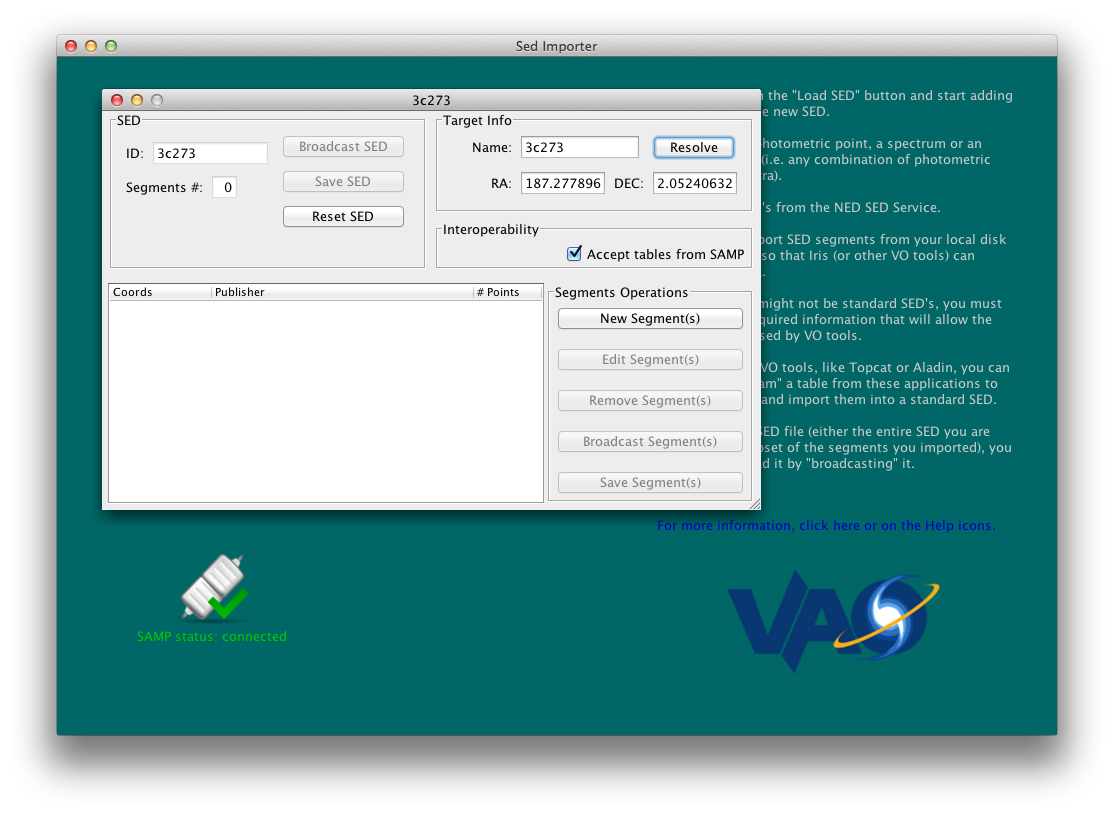
1. Start the Iris SED Importer tool, the SEDImporter.
2. Select Load SED. A text box will open; provide a name for the new SED (e.g., 3C273). A new window should appear, with the ID specified.
3. In the Target Info area, enter the name 3C273 to resolve the source name into coordinates. Select Resolve and the coordinates should be filled in. (RA = 187.277896334, DEC = 2.052406321).

1. At the time of the writing of this document, the Year 2 Fermi data has not been incorporated into the NASA Extragalactic Database (NED). We must, therefore, do it ourselves. Included in this tutorial should be a file named 3c273_fermi.dat containing the relevant Fermi data (Abdo et al. 2011).

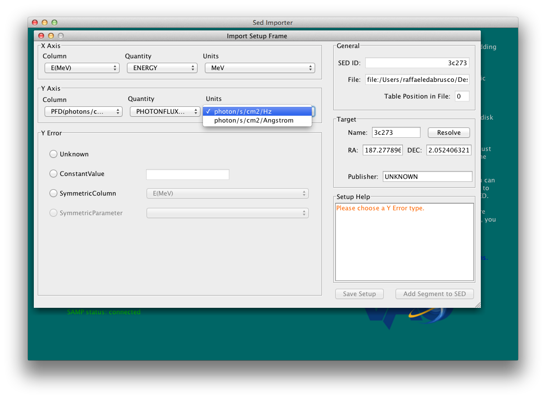
   1. Select New Segment to begin adding data. A new window should appear. Since we are loading Fermi data from an external file, ensure that the Location on Disk radio box is selected. Browse one’s disk to select the file, ensure that the File Format is ASCII Table, and then load the data.
   2. A new Import Setup window should appear. This step is necessary to tell Iris what the relevant units are. The external Fermi file should be structured so that the first column (col1) is energy in units of Mev, the second column is photon flux density in units of photons/cm2/s/Hz, and the third column contains the uncertainties as a SymmetricColumn. Because these data are being loaded from an external file, the Publisher is specified as UNKNOWN. For ease of keeping track of various data segments, it is recommended that one change this field to something meaningful, e.g., Fermi.
   3. Select Add Segment to SED.

2. At this point, the SED window should show a record listing 5 data from the publisher Fermi, with the coordinates of 3C273.

3. We now add the published data from NED. Select New Segment. A new window should appear, but this time select Get an SED from the NED Service. The target Name field should already be completed. Select Import NED SED, and a new listing should appear with 67 data from the publisher NASA/IPAC Extragalactic Database.

4. We now add our hypothetical data from ALMA. This time we won’t import the file directly into the SEDImporter from the file, but we will imagine the ALMA data have been retrieved from a VO service that searches tabular data, using TOPCAT. So, if you know how to use TOPCAT, import the second file 3c273_alma.dat into TOPCAT.

   1. Select the file in TOPCAT main window the file and sent it to the SEDImporter using the SAMP interoperability between the SEDImporter and TOPCAT (click on the icon with the radio tower).
   2. From this point on, the steps are similar to adding the Fermi data, but are listed here for completeness. A new Import Setup window should appear automatically when the file is “broadcast” from TOPCAT. The second column (col2) is frequency in units of GHz, the fourth column (col4) is flux density in units of Jy, and the fifth column (col5) is the uncertainties as a SymmetricColumn. Because these data are being loaded from an external file, the Publisher is specified as UNKNOWN. For ease of keeping track of various data segments, it is recommended that one change this field to something meaningful, e.g., ALMA.
   3. Select Add Segment to SED.

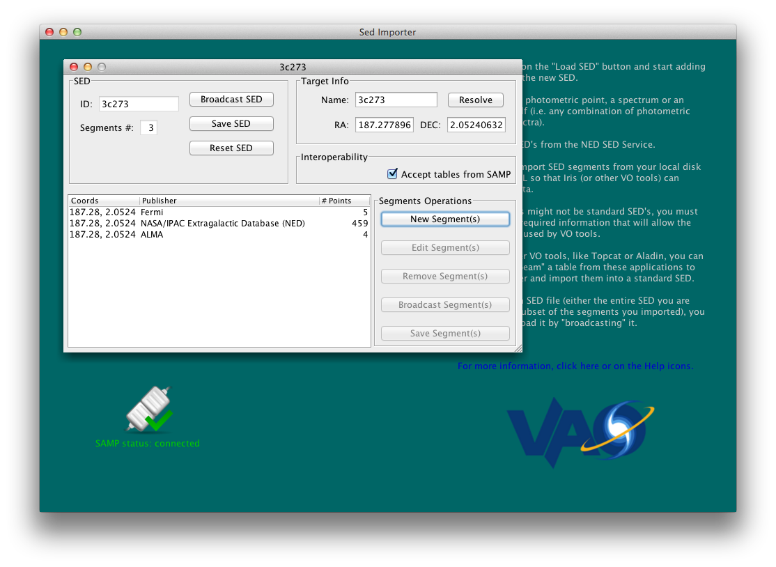
1. At this point, the SED window should show a record listing 4 data from the publisher ALMA, with the coordinates of 3C273.
2. Save this SED, which should contain 3 segments from the publishers Fermi, NASA/IPAC Extragalactic Database, and ALMA, to an external file. Save it as a VOTable (data/metdata formatted in XML).

Modeling the SED

1. In order to display this SED, click on Launch Iris icon from the main SEDImporter window. A new window should appear.

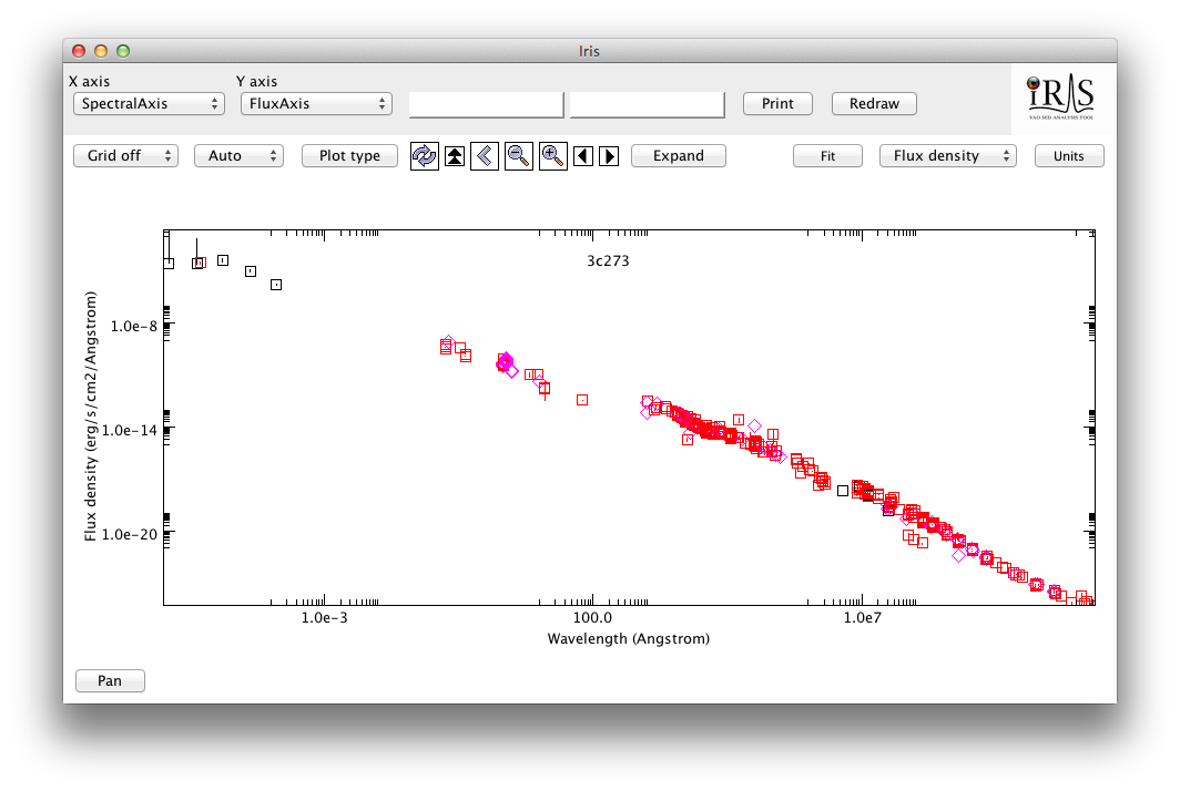
1. Go back to the main SED window of the SEDImporter and click on Broadcast SED to seamlessly send the whole SED to Iris. The plot of the SED should appear. Black boxes show data from the NED SED service, with purple associated to data points with no error estimates available. Red boxed show data contained in the two files that have been imported into the SEDImporter.
2. You can change the units of measure of the SED plot, zoom in or out or/and change the representation of the SED. For example, you can select Flux in the quantity selector that is by default set to density flux. You will be asked to select the units of measure for the spectral and flux axes, a good choice is Hz and Jy-Hz respectively for the nu*f(nu) visualization of the SED.

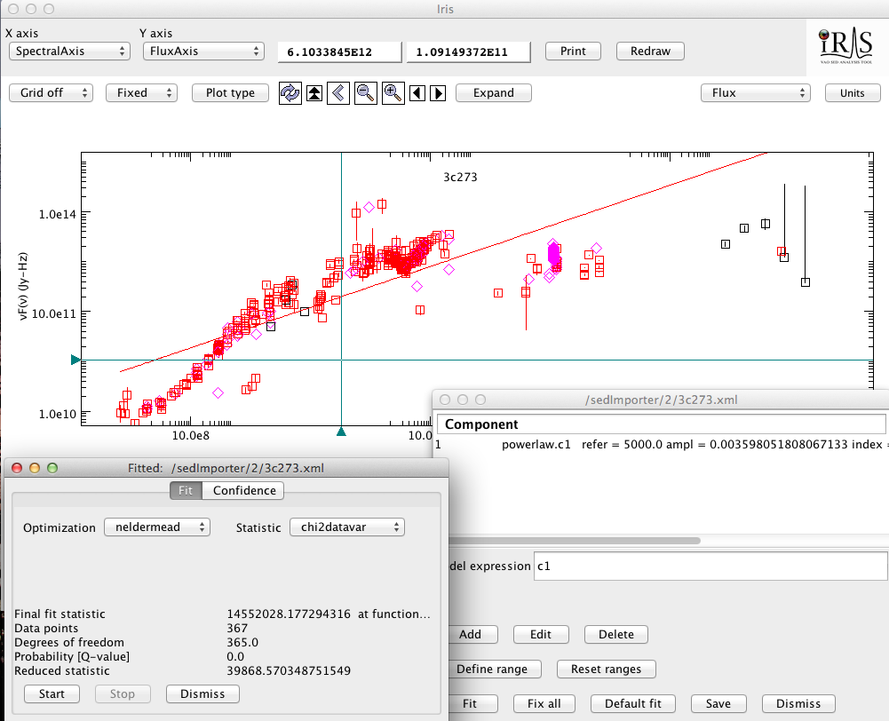
1. Clicking on Fit, you will see that the powerlaw model from the models list is added by default. You can click on Fit, pick an Optimization method and one Statistics and perform the fit with this model.
2. If you are not satisfied with the fit, you can edit the model. For example, select the powerlaw model and delete it by clicking on Delete, then click on the Add box to add another model. Select brokenpowerlaw (c1 component should be automatically added in the Model expression text field); you can use the broken powerlaw to perform a first fit by clicking again on Fit, then leave the fit statistic to its default value and change the optimization method to chi2davatar;
3. You can build an arbitrarily complex model function for the fit by mathematically combining the elementary function in the Model expression field. You can try to combine the brokenpowlaw model with other models to improve the fit of the SED of 3C273.
4. By selecting Define range in the main Fit window, you can interactively define the range of the fit by clicking on the two extremes of the range.
5. The custom fitted model parameters can be saved to a local file before exiting the fitting session, by selecting Write to a text file option from the File menu of the Fit window and then by clicking on Write active components.

Independent Exercise

In Iris, you can compare multiple SEDs by overplotting them. As an example, you can build the SED for a different source, say the blazar 4C+28.07 for which a decent amount of multiwavelength observations and Fermi data are available (provided in 4c28.07_fermi.dat). Try to build the SED for 4C+28.07 within the SEDImporter using both NED SED data and the Fermi data contained in the “4C+28.07_fermi.dat”, while Iris is still showing 3C273 SED. Then, send the newly created SED to Iris and overplot it to the previously plotted SED.

Note

If you can’t find out how to coplot SEDs, have a look at the official documentation.